Department of
Environmental Studies
Building environmental champions to help solve the planet’s most pressing problems.
The environment today is facing fundamental challenges calling for impactful solutions. More than ever before, the planet needs thinkers, analysts, and advocates who can bridge environmental knowledge and stewardship to help uncover and implement solutions by considering the human dimensions of environmental issues.
The Environmental Studies Department educates and empowers students with expertise in policy, communication, leadership, justice, and education to address environmental problems. Through the knowledge and skills students gain at ESF, they can contribute to building an ecologically sustainable and socially just world.
Meet the Chair
Theresa Selfa, Ph.D.
"If you’re passionate about protecting the planet and building a more sustainable and socially just future, then Environmental Studies is a great path to pursue. We go further than helping students understand the causes and impacts of environmental problems—we teach them how to solve these problems through environmental policy and decision-making processes."
Undergraduate Degree Programs
Environmental Education and Interpretation
Discover and design impactful ways to connect diverse learners with science and natural and built environments so that they can collaborate to care for our places.
Learn More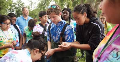
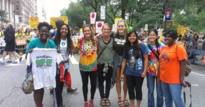
Environmental Studies
Preparing students with the knowledge and experience to work toward an ecologically sustainable and socially just world.
Department Career Outcomes
The expertise of our students have never been more in demand.
Our high placement rates mean students are prepared to transition from ESF undergraduate
to employment or graduate study.
Graduate Study
Get a M.S., or M.P.S. in Environmental Studies with Research Areas in
Environmental Communication
Environmental Policy
Get a Ph.D. in Environmental Studies
Get a fully online M.P.S. in Environmental Leadership, Justice & Communication
Three online certificates + a capstone project = M.P.S. Degree
Get a Graduate-Level Certificate of Advanced Study
Environmental Decision Making
Environmental Leadership (Online)
Science & Environmental Communication (Online)
Environmental Justice & Inequality (Online)