Department of
Sustainable Resources Management
At the forefront of defining professions that sustainably manage natural and built systems.
By studying and working to preserve and utilize our resources, we can help to better the environment while providing short- and long-term benefits for people. In the department of Sustainable Resources Management (SRM), students learn to use and sustainably manage renewable, natural, and constructed resources — such as energy, forests, soils, water, and building materials — from faculty who address these issues through applied and fundamental research, technology transfer, and teaching. Our program is designed to advance our understanding of current environmental issues through cutting-edge research, education, and outreach.
Meet the Chair
Christopher A. Nowak, Ph.D.
"Sustainability is at the forefront of discussions about the environment and climate change, and students seeking a program that addresses those needs will find it in SRM, where they learn from faculty who are recognized as among the best in the world."
Undergraduate Degree Programs
Construction Management
Designed to give you the tools you need to prepare for a rewarding career in sustainable construction.
Learn More
Forest Ecosystem Science
Learn the science and practice of sustaining forests on a rapidly changing planet.
Forest Resources Management
Master the knowledge and skills needed to conserve and manage forests and the environment.
Learn More
Natural Resources Management
Acquire skills to understand, analyze, and manage natural resources and systems.
Learn More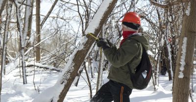
Sustainability Management
Enter the world where the science of sustainability meets real world applications.
Learn More
Sustainable Energy Management
Gain an understanding of responsible energy use and the development of sustainable energy sources.
Learn More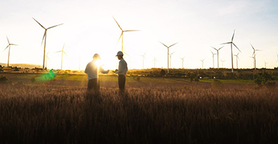
Learn more about our undergraduate programs
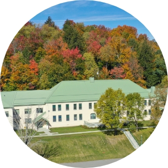
Associate Degree
Get an A.A.S. at the Ranger School (Wanakena, N.Y.)
Forest Technology
Land Surveying Technology
Environmental and Natural Resources Conservation
Department Career Outcomes
The expertise of our students have never been more in demand.
Our high placement rates mean students are prepared to transition from ESF undergraduate
to employment or graduate study.
Graduate Study
Get an M.S., M.P.S., or Ph.D. in Sustainable Resources Management
Forest Resource Management
Ecology and Ecosystems
Economics, Governance, and Human Dimensions
Forest Management & Silviculture
Monitoring, Analysis, and Modeling
Sustainable Construction Management
Construction Management
Sustainable Construction
Get a Masters of Forestry (M.F.) in Forest Management and Operations
Forest Management and Operations