Department of
Chemical Engineering
Meeting society's most pressing needs — sustainably.
Today’s society requires us to think differently about the way we do things. That’s why in the Department of Chemical Engineering, we create solutions that leave the world in a better place than we found it. We teach students in the classroom, in the laboratory, and at industrial locations how to build and implement sustainable processes, materials, and energy for a cleaner earth. Our program is designed at the forefront of modern chemical engineering, with a focus on developing high-tech — and planet-friendly — approaches to bioprocesses, biopharmaceuticals, and sustainable materials.

Meet the Interim Chair
Stephen Shaw, Ph.D.
" An engineering degree changes a person’s perspective on the world. Instead of seeing barriers, engineers see problems to be solved. An Environmental Resources Engineering degree gives students the skills to solve problems related to water and air pollution, climate change, resource production and recovery, environmental risk assessment, municipal infrastructure, and ecosystem restoration."
Undergraduate Degree Programs
Bioprocess Engineering
Pursue an exciting path in biopharmaceuticals — manufacturing drugs, vaccines, and therapies for diseases and health.
Learn More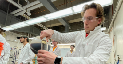
Chemical Engineering
Learn strategies to solve society’s critical challenges in future energy, manufacturing, and the environment.
Learn More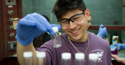
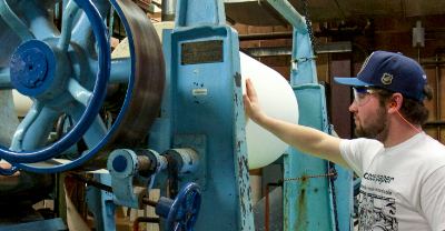
Paper Engineering
Develop and manufacture new and sustainable paper and packaging materials.
Department Career Outcomes
The expertise of our students have never been more in demand.
Our high placement rates mean students are prepared to transition from ESF undergraduate
to employment or graduate study.
Graduate Study
Get an M.S. or Ph.D.
Bioprocess Engineering
Paper Science and Engineering
Get an M.P.S.
Bioprocess Engineering
Paper Science and Engineering
Sustainable Engineering Management